Research Areas
Research Projects
Project Contact
Jeffreys Ledge
High Resolution Bathymetry, Surficial Sediment Maps and Interactive Database: Jeffreys Ledge and Vicinity
Contact: Larry Ward and Paul Johnson
Background
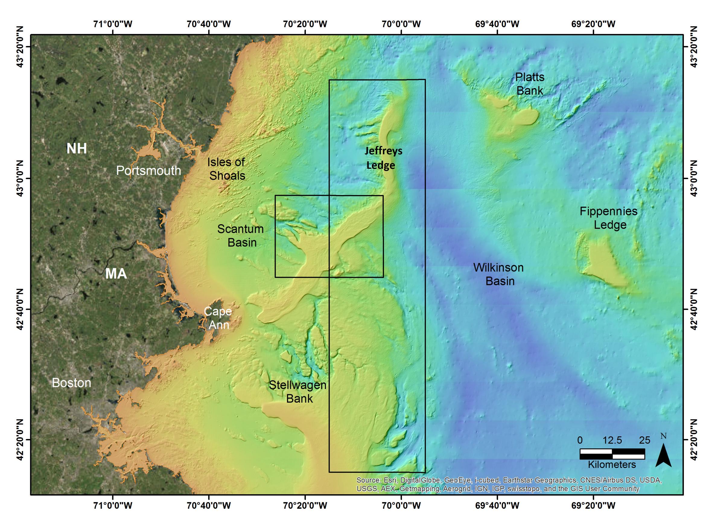
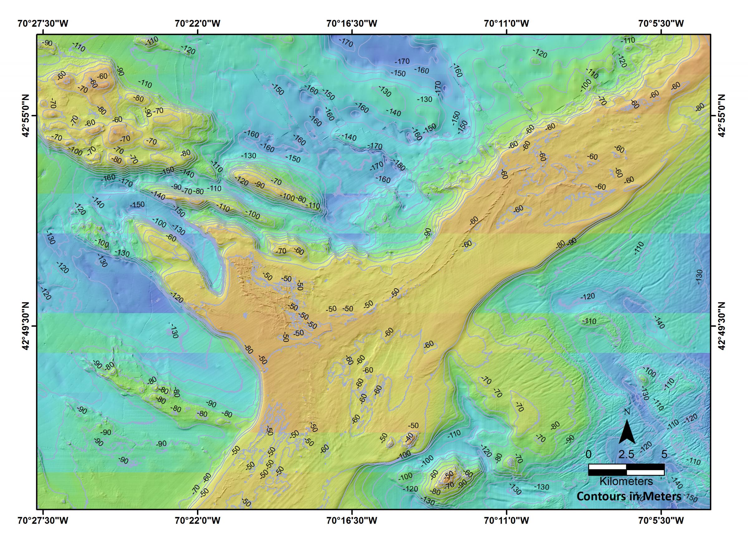
Jeffreys Ledge is a major morphologic feature in the western Gulf of Maine (WGOM) located ~50 km off the coast of New Hampshire, although coming within ~10 km of shore by Cape Ann, Massachusetts (Figure 1). Jeffreys Ledge rises as much as ~150 m from the adjacent basins (i.e., Scantum Basin or Wilkinson Basin) to depths less than 50 m on the ridge surface (Figure 2). It extends over 100 km along its north-northeast to south-southwest axes, while generally only being 5 to 10 km in width (~20 km maximum). Jeffreys Ledge and the surrounding region, like many features in the Gulf of Maine, most likely owes its origin and morphologic and sedimentologic features to a combination of fluvial erosion in the late Neogene (formerly Tertiary) leaving topographic highs, subsequent glaciations and sea-level fluctuations in the Quaternary, and late Pleistocene and Holocene marine processes (Uchupi 1966; Oldale and Uchupi 1970; Oldale et al. 1973; Ballard and Uchupi 1974; Schnitker et al. 2001, Uchupi 2004, Barnhardt et al. 2007, Uchupi and Bolmer 2008).
 |
|
Figure 1. Location map for the western Gulf of Maine. The study area is outlined by the smaller rectangle. The larger rectangle is the Western Gulf of Maine Closure. |
|
 |
|
Figure 2. Bathymetry of the study area (outlined by small rectangle on Figure 1) on Jeffreys Ledge. |
|
In 1998, the National Marine Fisheries Service established the WGOM Closure area which encompasses the northern and middle reaches of Jeffreys Ledge (Figure 1). The closure, one of the largest in the world, extends ~110 km north-south and is ~30 km in width. A year-round prohibition of bottom gillnets and otter trawls was implemented in an effort to help rebuild the groundfish stocks (e.g., cod, haddock, other gadids, and flatfish) in the WGOM, as well as to help protect habitat (Grizzle et al. 2009).
From 2002 to 2005, the University of New Hampshire (UNH) Center for Coastal and Ocean Mapping (CCOM) was part of an interdisciplinary effort to evaluate the effect of the WGOM closure on bottom habitats. The study focused on a ~18.5 by ~27.8 km area (~515 km²) on Jeffreys Ledge that encompassed similar seafloor types inside and outside of the closure (Figure 1). During this study, high resolution multibeam echosounder (MBES) surveys were completed, bottom sediment samples were collected and processed for grain size, and seafloor video was obtained along bottom transects.
Provided here are bathymetric maps of the study area (Figures 2 and 3), grain size data and sediment classifications based on the bottom sediment samples (Figure 4), a seafloor sediment classification based on the video and bottom photographs showing the characteristics of the seafloor (Figure 5 and 6), a surficial geology map of the study area (Figure 7), and an interactive map that allows the sediment grain size data, video classification data, and seafloor photographs be accessed (Figure 8).
Suggested Citation
The data and information provided here is available for general use, but the University of New Hampshire Center for Coastal and Ocean Mapping/Joint Hydrographic Center should be credited with the following citation:
Ward, L.G., R. Grizzle and P. Johnson. 2019. High Resolution Seafloor Bathymetry, Surficial Sediment Maps, and Interactive Database: Jeffreys Ledge and Vicinity. University of New Hampshire Center for Coastal and Ocean Mapping and Joint Hydrographic Center, Durham. http://ccom.unh.edu/project/jeffreys-ledge
Data Collection and Processing
Bathymetric Maps
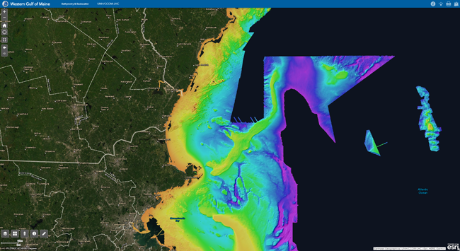
Over 85% of the UNH study area was surveyed under contract from UNH CCOM to Science Applications International Corporation (SAIC) in December 2002 using a Reson 8101 Multibeam Echo Sounder (MBES). Smaller (~2 by ~3 km), higher resolution MBES surveys were conducted within the original survey area at two sites by the National Oceanic and Atmospheric Administration (NOAA) Ship Thomas Jefferson in October 2003, using a Reson 8125 MBES. Standard hydrographic protocols were used during all surveys (NOAA Hydrographic Manual 1976). Data from both surveys were processed with CARIS HIPS/SIPS (v. 5.3) producing tide-, motion- and sound-speed-corrected, geo-referenced bathymetry. The MBES survey of the entire study area using the Reson 8101 was gridded at 5m, while the smaller survey areas surveyed with the Reson 8125 were gridded at 2m (Figure 2). These high resolution surveys have been incorporated into a broader bathymetry synthesis for the the Northeast focusing on the Western Gulf of Maine (see Figure 3).
|
|
Figure 3. Gulf of Maine Bathymetry and Backscatter Compilation. |
Bottom Sediment Sampling, Grain Size Analysis, and Classification
 |
|
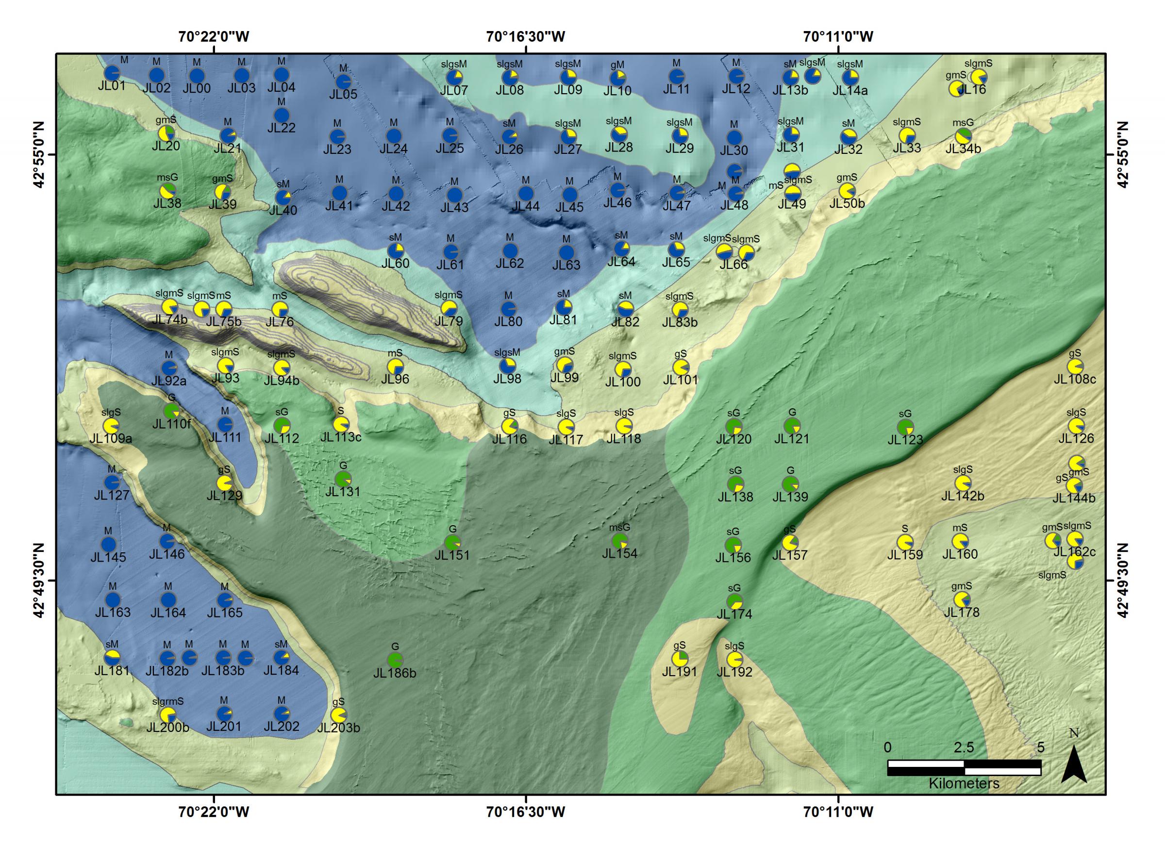
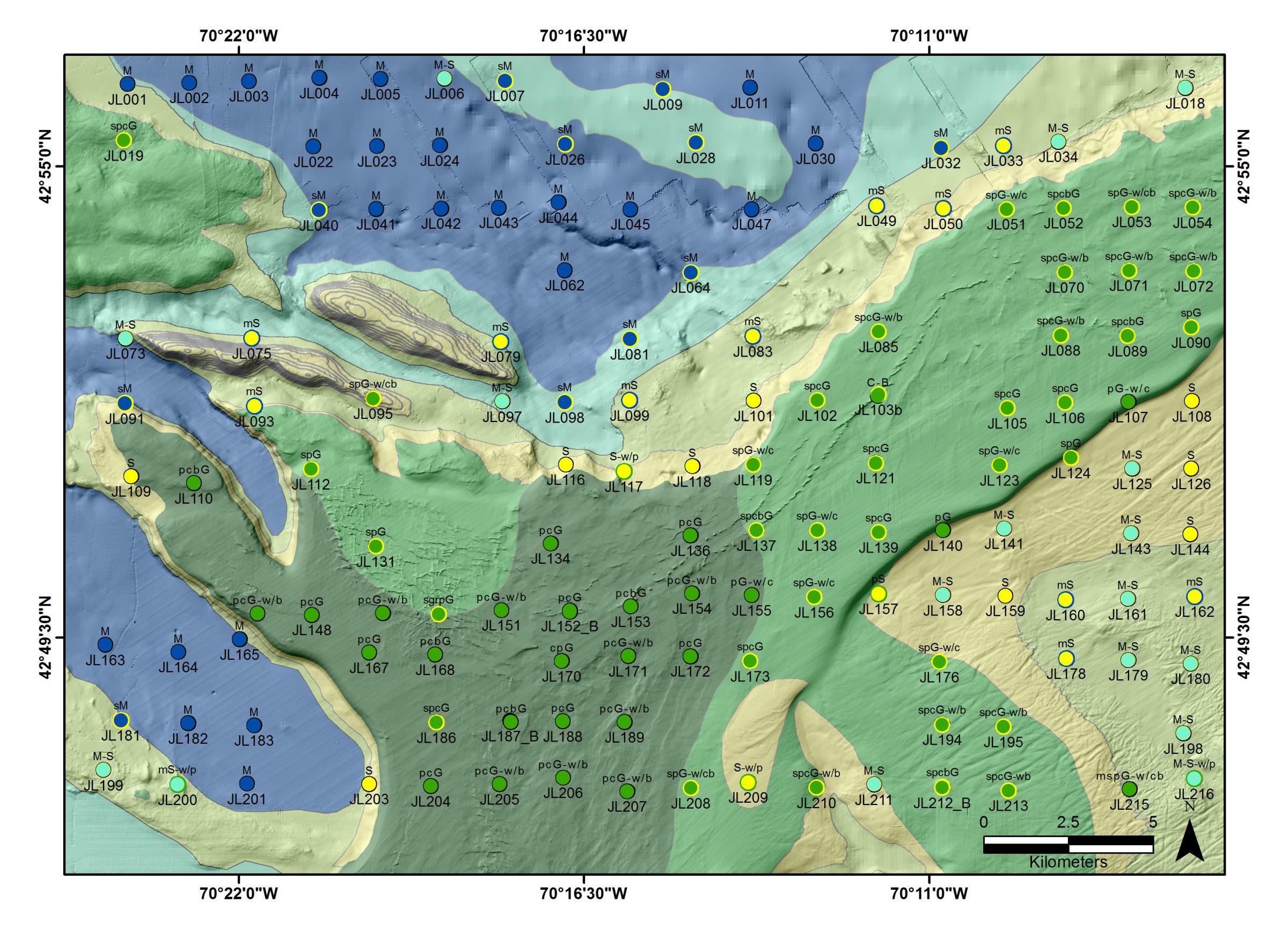
Figure 4. Station locations for the bottom sediment samples analyzed for grain size. The circles (station markers) show the percentage of gravel (green), sand (yellow), and mud (blue). The sediment classification (abbreviated) and station numbers are given above and below (respectively) the station markers. Complete grain size statistics can be viewed with the interactive map at the end of this page. The base map depicts the surficial sediment distribution and is explained below. |
|
Bottom sediment samples were collected at 124 stations (Figure 4) from 2002 to 2005 (primarily in 2002) largely using chartered fishing vessels. Samples were obtained with either a Shipek grab sampler (0.04 m² sampling area) or a Wildco box corer (0.0625 m² sampling area). Grain size was determined using standard sieve and pipette analytical techniques (Folk 1980).
The grain size data was analyzed in “Gradistat” (Blott and Pye 2001) and the major statistics (mean, sorting, skewness, and kurtosis) were determined based on the distribution of phi sizes as recommended in Folk and Ward (1957). The sediment classification (name) is presented using the Wentworth Scale (as discussed in Folk 1980) and the modifications recommended by Blott and Pye (2001), which primarily effects the gravelly sediments and the silt-clay boundary. Organic content was estimated by loss-on-ignition (% LOI) after four hours at 450°C.
Seafloor Video Acquisition and Analysis
 |
|
Figure 5. Locations of video stations at Jeffreys Ledge. The circles (station markers) color indicates general sediment classification based primarily on video (solid green is gravel; green with yellow halo is sandy gravel; yellow is sand; blue is mud; and cyan is sand or mud). The complete sediment classification (abbreviated) based on video is given above the station markers; the station number is given below the station marker. The base map depicts the surficial sediment distribution and is explained below. Complete video-based classifications and bottom images can be viewed on the interactive map at the end of this page. |
|
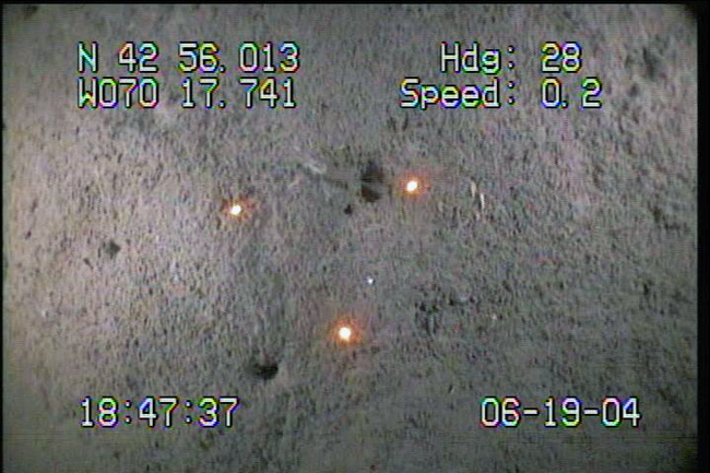
Seafloor videography was collected at the 141 stations (Figure 5) with a DeepSea Power and Light Multi SeaCam® 2050 housed in a constructed aluminum frame with synchronized strobe lights (Perkin Elmer Optoelectronics MVS-5000-CE96 Machine Vision Strobes) and an integrated positioning system (Sea-Track Video Overlay). The Multi Seacam®2050 has a f3.5 wide angle lens with a fixed focus, a depth of field of 10 cm to infinity, and a field of view in water of 79° (H) by 59° (W). The position recorded the location of the support vessel using an onboard differential GPS. The camera was suspended within ~50 cm of the bottom and six to ten minutes of downward looking near-vertical video normally recorded at each station as the support vessel drifted. Periodically, the camera was allowed to touch down on the bottom providing vertical views. Three lasers, positioned in a triangular pattern 10 cm apart around the camera lens, were visible on the bottom and allowed quantitative measurements to be made.
Seafloor Sediment Classification Based on Video
A descriptive classification for the bottom sediment was developed for this study primarily based on visual inspection of the video and an estimation of grain size (with the aid of the lasers). At each station, a portion of the video transect that typically extended approximately 25 to 50 m in length was isolated for analysis. In some instances, this length of useable video was not available due to field conditions and a shorter distance was analyzed. Subsequently, the video was subsampled to approximately one frame per second and consecutive frames that did not overlap analyzed. The number of frames analyzed per station varied depending on the length and quality of the video transect and ranged from 4 (for stations that were subsampled due to unusual features such boulder fields) to 81. However, ~75% of the stations had between 20 to 56 frames analyzed.
Bottom sediment viewed in each frame was first described as mud-sand or gravel. The camera optics did not allow individual particles of mud or sand be seen. Therefore, the sediment type was considered a mud-sand if individual grains were not visible and little or no gravel was present. The mud-sand class was not differentiated into mud, sandy mud, muddy sand or sand unless a bottom sediment sample was collected nearby (<100 m), grain size analysis was conducted, and the seafloor was relatively homogeneous. Gravel bottoms were typically composed of mixtures of pebbles, cobbles, and boulders with varying amounts of sand or granule material. If the gravel size clasts (individual grains or fragments of a rocks that were visible) were largely in contact, the bottom was classified as a gravel with the appropriate modifiers (described below and in Table 1). If the gravel clasts were separated by sand or granule material, then the seafloor was classified as a sandy gravel with the appropriate modifiers.
Table 1. Classification of gravel bottoms based on videography from Jeffreys Ledge.
| Seafloor Classification |
Gravel in Contact or Separated by Sand |
% of Frames with Pebbles | % of Frames with Cobbles | % of Frames with Boulders |
| Pebble Gravel | Gravel in Contact | > 50 % | < 10 % | < 10 % |
| Pebble Gravel with Cobbles | Gravel in Contact | > 50 % | 10 – 50 % | < 10 % |
| Pebble Gravel with Cobbles and Boulders | Gravel in Contact | > 50 % | 10 – 50 % | 10 – 50 % |
| Pebble and Cobble Gravel | Gravel in Contact | > 50 % | > 50 % | < 10 % |
| Pebble and Cobble Gravel with Boulders | Gravel in Contact | > 50 % | > 50 % | 10 – 50 % |
| Pebble Cobble and Boulder Gravel | Gravel in Contact | > 50 % | > 50 % | > 50 % |
| Sandy Pebble Gravel | Separated by Sand | > 50 % | < 10 % | < 10 % |
| Sandy Pebble Gravel with Cobbles | Separated by Sand | > 50 % | 10 – 50 % | < 10 % |
| Sandy Pebble Gravel with Cobbles and Boulders | Separated by Sand | > 50 % | 10 – 50 % | 10 – 50 % |
| Sandy Pebble and Cobble Gravel | Separated by Sand | > 50 % | > 50 % | < 10 % |
| Sandy Pebble and Cobble Gravel with Boulders | Separated by Sand | > 50 % | > 50 % | 10 – 50 % |
| Sandy Pebble Cobble and Boulder Gravel | Separated by Sand | > 50 % | > 50 % | > 50 % |
To further refine the gravel classification, the presence (or absence) of pebbles, cobbles, or boulders within each frame (that did not overlap) for a station was noted and the percentage of frames containing each of these categories for the entire station transect determined. Note that the actual percentage of the area of a frame composed by a class size (pebble, cobble, or boulder) was not determined, rather simply if any pebbles, cobbles, or boulders were present in that frame. For this study, a pebble was defined as any individual clast that was large enough to visible in the video and smaller than ~6 cm as determined by comparison to the lasers; cobbles were ~ 6 to ~25 cm; and boulders were larger than ~25 cm. These boundaries approximate the Wentworth scale (pebbles: 4 to 6.4 mm; cobbles: 6.4 to 25.6 cm; and boulders: >25.6 cm; see Folk 1980). Granule size gravel (2 to 4 mm) was not identified due to the limitations of the camera optics.
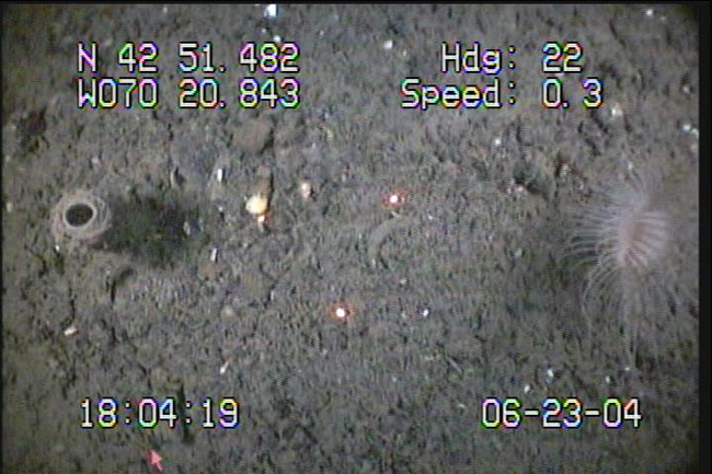
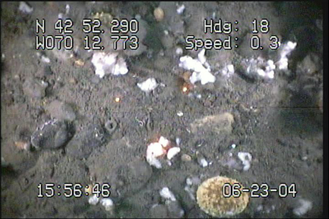
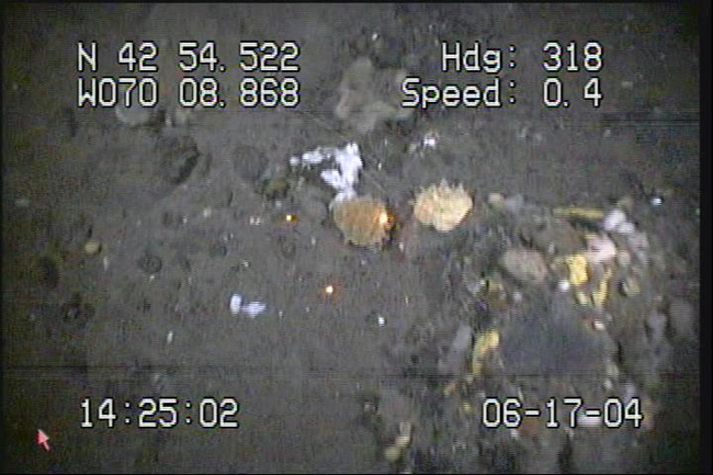
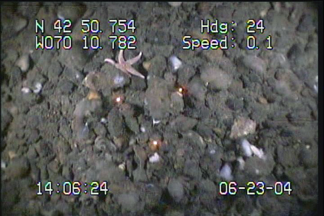
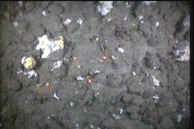
The classification of the gravel substrate was based on the percentage of frames analyzed at a station that contained pebbles, cobbles, or boulders. If any of these size clasts were found in over 50% of the frames analyzed, then the seafloor was considered a pebble, cobble, and/or boulder gravel. If these clasts appeared in 10 to 50% of the frames analyzed, then the seafloor was considered a gravel with pebbles, cobbles, and or boulders. A gravel bottom could then be any combination of these sizes. For instance, a pebble gravel, a pebble gravel with cobbles, or a pebble cobble gravel with boulders, depending on the occurrence of the different clast sizes. See Table 1 for classification and Figure 6 for examples.
 |
 |
 |
JL112 - Sandy Pebble Gravel |
JL102 - Sandy Pebble Cobble
|
JL052 – Sandy Pebble Cobble
|
 |
 |
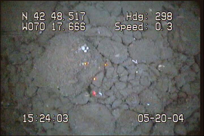 |
JL140 – Pebble Gravel |
JL134 – Pebble Cobble Gravel |
JL187a – Pebble Cobble Boulder
|
 |
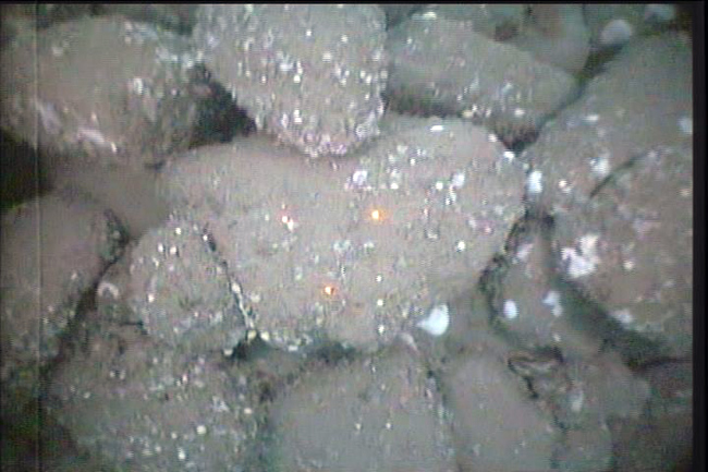 |
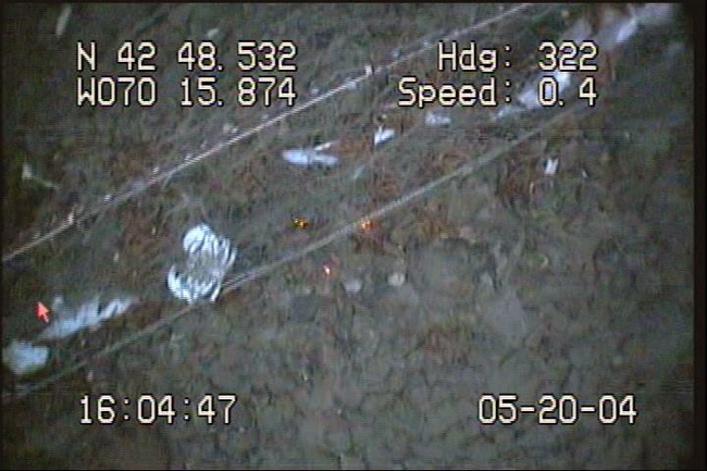 |
JL007 – Sandy Mud |
JL152a – Cobble Boulder Ridge |
JL189 – Pebble Cobble Gravel with Boulders. Note ghost net. |
|
||
Summary
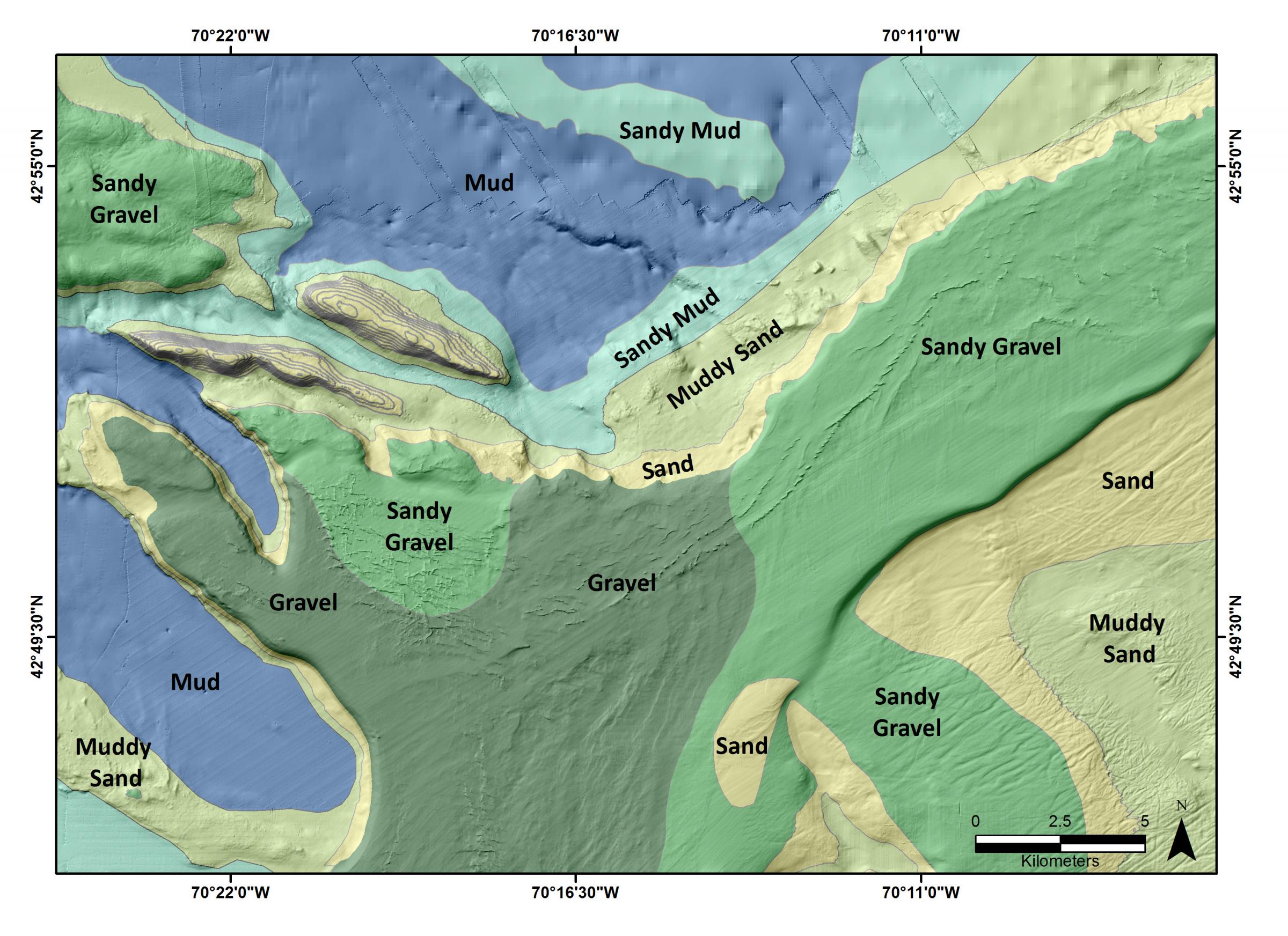 |
|
Figure 7. Surficial sediment map for the study area (small rectangle in Figure 1). Two small areas showing contours were not mapped. |
|
High-resolution bathymetry, videography, and direct sampling were used to develop detailed descriptions of the morphology and surficial sediments (size, classification and distribution) of the seafloor for a ~515 km² area at Jeffreys Ledge. A sediment classification based on video for gravel dominated areas (i.e., platform or surface of Jeffreys Ledge based on video), used in conjunction with conventional bottom sediment sampling and analysis in finer-grained sediments (i.e., deeper adjacent areas), facilitated the development of the bottom sediment map (Figure 7). This knowledge, along with the high-resolution bathymetry, is important to managing this environment, as well as understanding the geologic processes at play in and around Jeffreys Ledge.
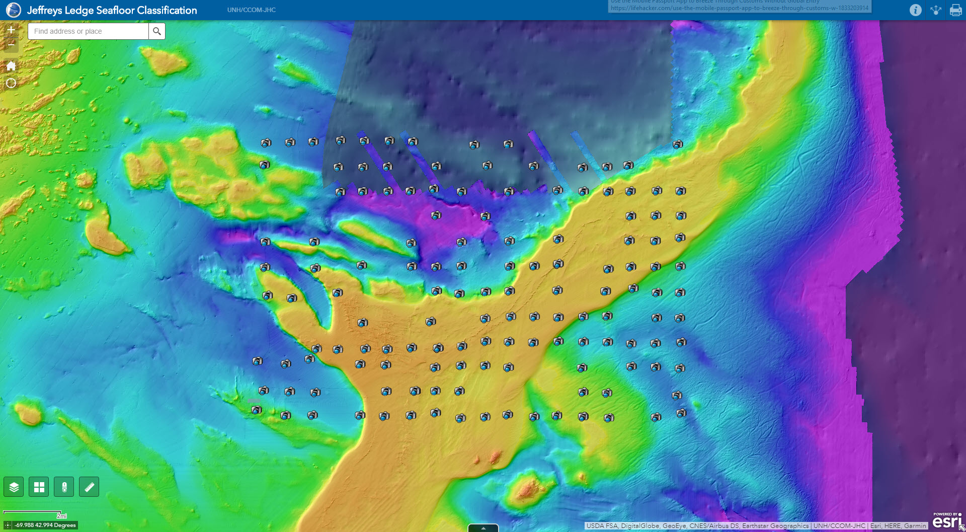
Interactive Base Map
The interactive base map facilitates access to the grain size data, sediment classifications, and bottom photographs of the ~515 km² area of the seafloor studied by UNH at Jeffreys Ledge. Click on the map to connect to the interactive map. The different databases can be viewed by clicking on the icon on the lower left of the figure, choosing the layer of interest, and clicking on a station symbol.The sediment statistics are shown in pop-up windows for all stations. In the Seafloor Photos & Classification layer, the links to the bottom photographs are found under “Attachments.” Simply click on the jpg file of interest.
*** Click the image below to access the interactive map. ***
Acknowledgements
This research was supported by UNH/NOAA Joint Hydrographic Center Award NA10NOS4000073, the UNH Northeast Consortium (NEC), and the UNH Atlantic Marine Aquaculture Center (AMAC). The bottom sediment samples were collected under the direction of Dr. Raymond Grizzle (UNH School of Marine Science and Ocean Engineering, Jackson Estuarine Laboratory). Much of the video was analyzed by Melissa Brodeur. Fishing vessels were used on all research cruises and included vessels captained by P. Kendall, C. Mavrikis, and J. Driscoll.
Publications from Research at Jeffreys Ledge
Ward, L., P. Johnson, M. Malik and R. Grizzle. 2014. Depositional environments of Jeffreys Ledge, Western Gulf of Maine: Impacts of glaciation, sea-level fluctuations and marine processes assessed using high resolution multibeam bathymetry, subbottom seismics, videography, and direct sampling. American Geophysical Union Meeting, December 15-19, San Francisco, CA, EOS Transactions. AGU Fall Meet. Suppl., Abstract OS31A-0975.
Grizzle, R.E., L.G. Ward , L.A. Mayer, M.A. Malik, A.B. Cooper, H.A. Abeels, J.K. Greene, M.A. Brodeur and A.A. Rosenberg. 2009. Effects of a large fishing closure on benthic communities in the western Gulf of Maine: Recovery from the effects of gillnets and otter trawls. Fishery Bulletin 107:308-317.
Malik, M.A. 2005. Identification of Bottom Fishing Impacted Areas Using Multibeam Sonar and Videography. M.S. Thesis, University of New Hampshire, Durham. 125 pp.
Malik, M. A. and L.A. Mayer. 2007. Investigation of seabed fishing impacts on benthic structure using multibeam sonar, sidescan sonar, and video. ICES Journal of Marine Science 64: 1053–1065.
Ward, L.G., M.A. Malik, G.R. Cutter, M.A. Brodeur, R.E. Grizzle, L.A. Mayer and L. Huff. 2006. High resolution benthic mapping using multibeam sonar, videography, and sediment sampling in the Gulf of Maine: Application to geologic and fisheries research. Geological Society of America Abstracts with Programs, volume 38, number 7, p. 377.
Other References Cited in this Report
Ballard, R.D. and E. Uchupi. 1974. Geology of Gulf of Maine. American Association of Petroleum Geologists Bulletin 58:1156-1158 (No. 6, Part II of II).
Barnhardt, W.A. 2007. High-resolution geologic mapping of the inner continental shelf: Cape Ann to Salisbury Beach, Massachusetts. United States Geological Survey Open-File Report 2007-1373. 44 pp.
Blott, S.J. and K. Pye. 2001. Gradistat: A grain size distribution and statistics package for the analysis of unconsolidated sediments. Earth Surface Processes and Landforms 26:1237-1248.
Folk, R. L. 1980. Petrology of Sedimentary Rocks. Hemphill Publishing Company, Austin, TX. 182 pp.
Folk, R.L. and W.C. Ward. 1957. Brazos River bar: A study in the significance of grain size parameters. Journal of Sedimentary Petrology (now Journal of Sedimentary Research) 27:3-26.
NOAA Hydrographic Manual. 1976. NOAA/NOS Hydrographic Manual, 4th edition. US Department of Commerce, Washington, DC.
Oldale, R.N. 1985. Upper Wisconsinan submarine end moraines off Cape Ann, Massachusetts. Quaternary Research 24:187-196.
Oldale, R.N. and E. Uchupi. 1970. The glaciated shelf off Northeastern United States. United States Geological Survey Professional Paper 700B, pp B167-B173.
Oldale, R.N., E. Uchupi and K.E. Prada. 1973. Sedimentary Framework of the Western Gulf of Maine and Southeastern Massachusetts Offshore Area. U.S. Geological Survey Professional Paper 757. 10pp.
Schnitker, D., D.F. Belknap, T. Bacchus, J.K. Friez, B.A. Lusardi and D.M. Popek. 2001. Deglaciation of the Gulf of Maine. In: T.K. Weddle and M.J. Retelle (eds.), Deglacial History and Relative Sea-Level Changes, Northern New England and Adjacent Canada. Geological Society of America Special Paper 351, pp. 9-34.
Uchupi, E. 1966. Structural framework of the Gulf of Maine. Journal of Geophysical Research 71:3013-3028.
Uchupi, E. 2004. The Stellwagon Bank region off eastern Massachusetts: A Wisconsin glaciated Cenozoic sand bank/delta? Marine Geology 204:325-347.
Uchupi, E. and S.T. Bolmer. 2008. Geologic evolution of the Gulf of Maine. Earth-Science Reviews 91:22-76. doi:10.1016/j.earscirev.2008.09.002.


